Digital Portfolio

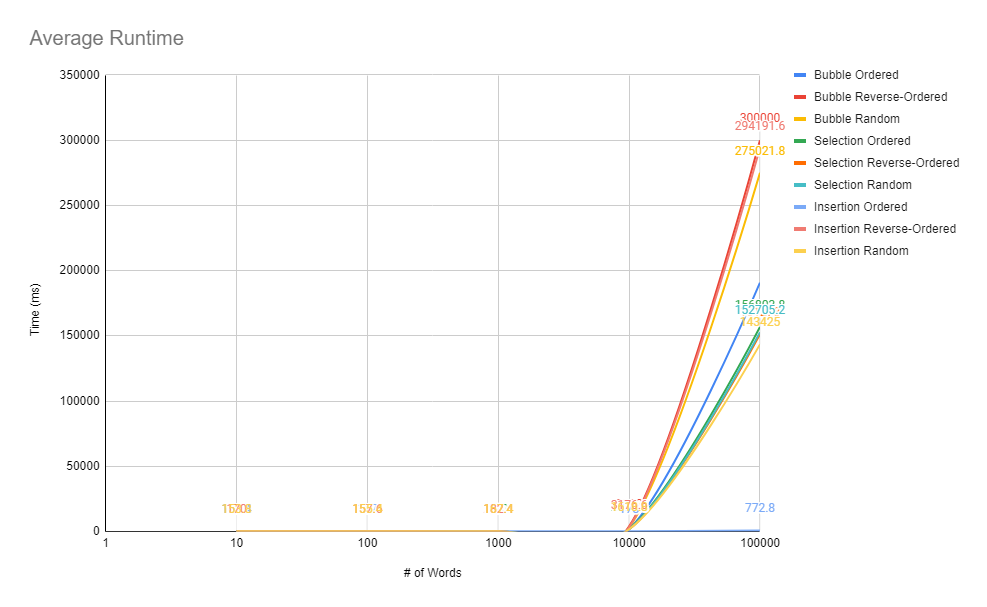
My graph provides a visual representation of data on average runtime for three different sorting algorithms (bubble sort, selection sort, and insertion sort) to sort three different types of text files (an ordered list of words, a reverse ordered list of words and a random list of words). The graph is organized with a horizontal axis for the number of words that were sorted and a vertical axis for the time, in milliseconds, it took each sorting algorithm to finish sorting the words. Additionally, the graph contains nine different lines to represent each sort and how it was used. For example, the green line (selection ordered) represents the tests where selection sort was used to sort an ordered list of words.
    As seen on the graph, the lines all exponentially grow. This can be explained by the fact that all three sorting algorithms have an average time complexity of θ(n^2). This means that on average, each algorithm should have a runtime that changes proportionately with n (the input size) squared. This also explains why the line drastically increases after ten thousand words are tested.
    From the data collected for the ordered list of words, we can see that insertion sort and bubble sort are faster than selection sort. This is because this is the best-case scenario for both bubble and insertion sort. With an already-ordered list of words, bubble sort will not have to perform any swaps, meaning that there will only be one pass. This makes bubble sort’s best-case time complexity O(n) as the runtime is directly proportional to n. The same time complexity can be applied to insertion sort as insertion sort will not have to perform any swaps and make only one comparison with an already ordered list of words. On the other hand, selection sort’s time complexity will remain at O(n^2) despite having an already ordered list of words. This is because selection sort will still have to perform n comparisons in n passes, as the sorting algorithm looks for the minimum values for each pass.
    On the contrary, it can be observed from the data collected for the reversed list of words that selection sort was faster than both bubble and insertion sort. This is because both bubble and insertion sort have to perform the most possible comparisons and swaps when presented a reverse-ordered list of words, making it the worst-case time complexity. However, selection sort remains consistent with the same time complexity it had with the ordered list of O(n^2) because it always makes n comparisons while looking for the minimum value of all n passes. This makes selection sort the best option for sorting a reverse-ordered list of words.
    It can be observed from the data collected for the random list of words that insertion sort was the fastest, selection sort was in the middle, and bubble sort was the slowest. This is because insertion sort will only perform the required amount of comparisons and swaps in n amount of passes. Whereas selection sort will have n^2 comparisons and n swaps. On the other hand, bubble sort is the slowest because it will perform n^2 comparisons and potentially n^2 swaps as well. These values can always vary because the list of words are random, meaning that the some list of words can potentially be more sorted than others. However, my data is consistent and valid because I used the same random list of words for each sort.
    In conclusion, we can determine that insertion sort is the fastest sorting algorithm (excluding the impractical reverse-ordered test), selection sort is the second fastest sorting algorithm, and bubble sort is the slowest sorting algorithm. This conclusion can be made based on the data I collected because the data I collected corresponds to each sorting algorithm’s time complexity, which validates the data I have collected.